mebioda

Inferences from tree shape

The birth/death process revisited

Nee, S, May, RM & Harvey, PH, 1994. The reconstructed evolutionary process. Philos Trans R Soc Lond B Biol Sci 344:305-311

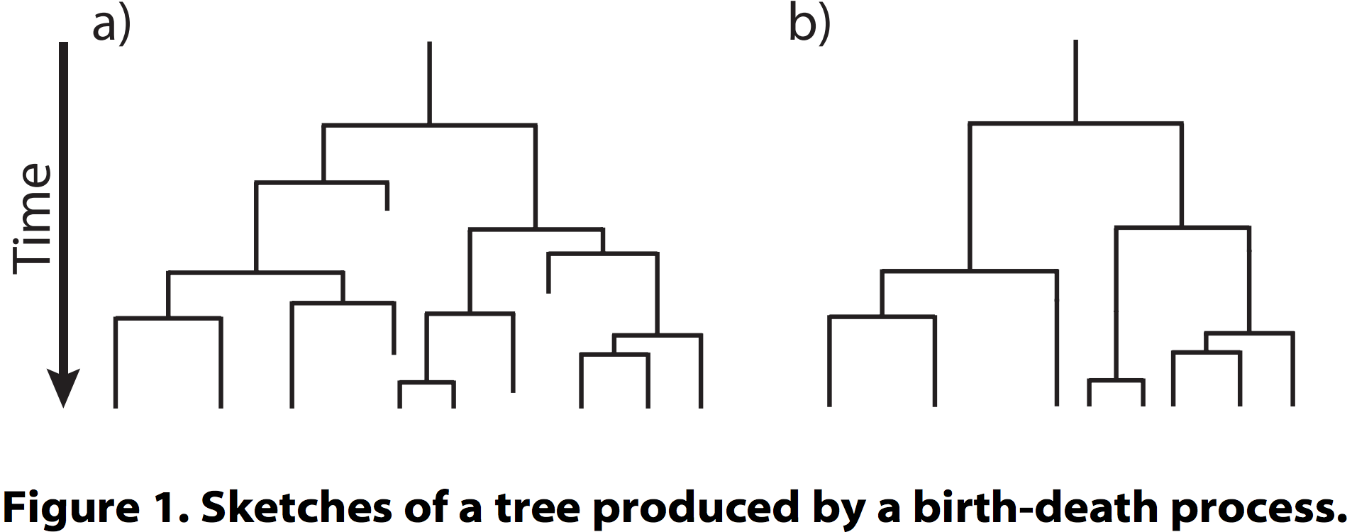
• In the simplest case, there are two constant parameters: speciation rate (lambda, λ) and extinction rate (mu, μ)
• Maximum likelihood estimation using the method of Nee et al. (1994) optimizes over μ/λ (or d/b, turnover) and λ-μ (b-d, net diversification)

Estimating birth/death parameters in ape

MLE of λ and μ can be obtained, for example, using ape in R:

library(ape)
phy <- read.tree(file="PhytoPhylo.tre")

# make tree binary and ultrametric
binultra <- multi2di(force.ultrametric(phy, method = "extend"))

# fit birth/death
birthdeath(binultra)

Resulting in:

Estimation of Speciation and Extinction Rates
            with Birth-Death Models

     Phylogenetic tree: binultra 
        Number of tips: 31389 
              Deviance: -392698.6 
        Log-likelihood: 196349.3 
   Parameter estimates:
      d / b = 0.9279609   StdErr = 0.001968166 
      b - d = 0.02020561   StdErr = 0.0005033052 
   (b: speciation rate, d: extinction rate)
   Profile likelihood 95% confidence intervals:
      d / b: [0.9265351, 0.9293592]
      b - d: [0.01985037, 0.02056618]

Estimating birth/death parameters in phytools

library(phytools)
phy <- read.tree(file="PhytoPhylo.tre")

# make tree binary and ultrametric
binultra <- multi2di(force.ultrametric(phy, method = "extend"))

# fit birth/death
fit.bd(binultra)

Resulting in:

Fitted birth-death model:

ML(b/lambda) = 0.2805 
ML(d/mu) = 0.2603 
log(L) = 196349.2855 

Assumed sampling fraction (rho) = 1 

R thinks it has converged.

Quick sanity check

Save for some differences in rounding, the results are identical:

• Log likelihoods are ± identical: 196349.3 (ape), 196349.2855 (phytools)
• μ/λ = 0.9279609 (ape), 0.2603/0.2805 = 0.927985739750446 (phytools)
• λ-μ = 0.02020561 (ape), 0.2805-0.2603 = 0.0202 (phytools)

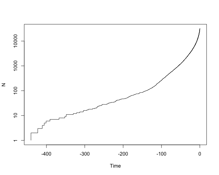
library(phytools)
phy <- read.tree(file="PhytoPhylo.tre")

# make tree binary and ultrametric
binultra <- multi2di(force.ultrametric(phy, method = "extend"))

ltt.plot(binultra,log="y")

Resulting in:

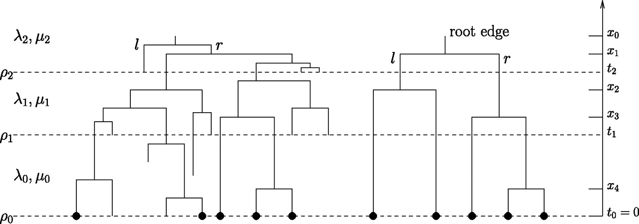
Is rate constant through time?

Stadler T, 2011. Mammalian phylogeny reveals recent diversification rate shifts. PNAS 108(15): 6187–6192

• Maybe diversification rates globally change as a function of some environmental variable, e.g. climate
• In this model, speciation (λ) and extinction (μ) can have different value within different time windows
• To allow for incomplete extant taxon sampling, an additional parameter (rho, ϱ) captures the completeness of the sampling

library(phytools)
library(TreePar)
phy <- read.tree(file="PhytoPhylo.tre")

# make tree binary and ultrametric
binultra <- multi2di(force.ultrametric(phy, method = "extend"))

# assume a near complete tree, rho[1]=0.95
rho <- c(0.95,1)

# set windows of 100myr, starting 0, ending 400myr
grid <- 100
start <- 0
end <- 400

# Vector of speciation times in the phylogeny. Time is measured 
# increasing going into the past with the present being time 0. 
# x can be obtained from a phylogenetic tree using getx(TREE).
x <- getx(binultra)

# estimate time, lambda, mu
res <- bd.shifts.optim(x,c(rho,1),grid,start,end)[[2]]

Interpreting the results

The result object looks like this:

> res
[[1]]
[1] 9.726584e+04 9.315585e-01 2.021164e-02

[[2]]
[1] 9.724484e+04 9.265107e-01 9.788873e-01 2.160713e-02 8.541232e-03 1.000000e+02

[[3]]
[1] 9.724243e+04 9.263011e-01 9.811704e-01 9.786497e-01 2.164689e-02 7.707626e-03 3.369398e-02
[8] 1.000000e+02 4.000000e+02

The MLE of a single rate shift is:

> res[[2]][6]
[1] 100

The rate before the shift is:

> res[[2]][5]
[1] 0.008541232

The rate after the shift is:

> res[[2]][4]
[1] 0.02160713

Is the result significant?

Test if one shift explains the tree significantly better than no shifts: if test > 0.95 then one shift is significantly better than 0 shifts at a 5% error:

> i<-1
> test<-pchisq(2*(res[[i]][1]-res[[i+1]][1]),3)
> test
[1] 1

How about two shifts?

> i<-2
> test<-pchisq(2*(res[[i]][1]-res[[i+1]][1]),3)
> test
[1] 0.8152525

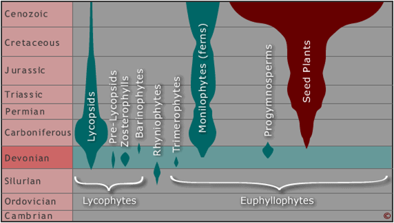
So, we estimate a single rate shift at 100MYA, with a low net diversification rate before the shift, and a higher rate afterwards. This meshes with our LTT plot and our general understanding of the diversification of seed plants:

Density-dependent diversification

DL Rabosky & IJ Lovette, 2008. Density-dependent diversification in North American wood warblers. Proc. R. Soc. B 275:2363-2371

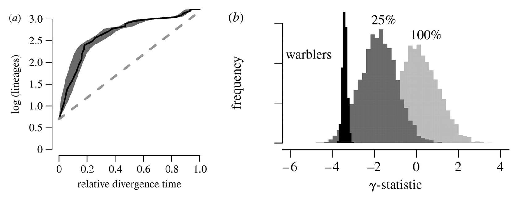
• (a) Log-lineage through time (LTT) plot for North American wood warblers. Black line indicates LTT curve for the MCC tree (figure 1), and grey shading indicates 95% quantiles on the number of lineages at any point in time as inferred from the posterior distribution of phylogenetic trees sampled with MCMC. The dashed line indicates expected rate of lineage accumulation under constant-rate diversification with no extinction. Lineages accumulate quickly in the early phases of the radiation relative to the constant-rate diversification model.
• (b) Posterior distribution of the γ-statistic for wood warblers (black) in comparison with the corresponding null distributions, assuming either complete (f=1) or incomplete (f=0.25) sampling. Negative values of γ relative to the null distribution indicate decelerating diversification through time.

More exercises with simulated data are here.

This site is open source. Improve this page.