mebioda
Phylogenetic comparative analysis
The problem: non-independence in comparative analysis
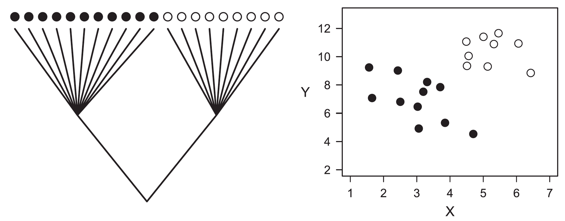
The problem of analyzing phylogenetically structured data with conventional statistical methods. Ignoring phylogeny, one would conclude that X and Y are positively correlated (Pearson r = 0.48, 2-tailed P = 0.034), when in fact this relationship emerges primarily from the high divergence in X and Y between the two clades at the root of the phylogeny.
False positives (type I errors)
Increased type I error rates of conventional statistics in analyses of interspecific data. When two traits evolve independently along a phylogeny according to Brownian motion, the probability of rejecting the null hypothesis of no correlation (type I error) increases with the amount of phylogenetic structure of the data.

Simulations with a star phylogeny result in the error rates of 5%, which is the expected type I error rate if conventional (nonphylogenetic) analyses are used.
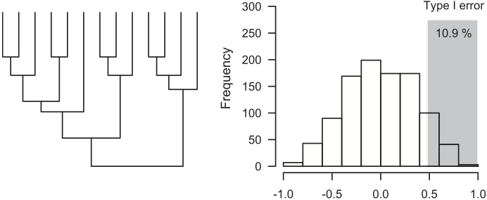
The shaded area represents simulations where the resulting ordinary Pearson coefficient falls above the tabular critical value of +0.476 (11 degrees of freedom), which would incorrectly suggest that the two traits are correlated.
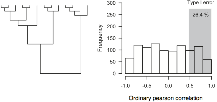
Type I error rates can be higher than 25% if the data shows a strong phylogenetic structure.
Brownian motion

- A hypothetical phylogeny representing the evolutionary relationships among five species, and its consequences at the level of phenotypic variation. Given the hierarchical patterns of relatedness among species, phenotypic data in comparative studies may not necessarily provide independent sources of information, as shown for the two pairs of closely related species that are phenotypically very similar.
- Consequently, patterns of phenotypic resemblance may be interpreted as evidence of evolutionary convergence (adaptation) when in fact they reflect common ancestry.
- For this particular example, phenotypic evolution proceeded as a random walk (i.e., a Brownian motion model of evolution).
Brownian simulation
Here is some code to perform discrete-time (non-phylogenetic) Brownian motion simulation:
# discrete time BM simulation
n<-100; t<-100; sig2<-1/t # set parameters
time<-0:t
X<-rbind(rep(0,n),matrix(rnorm(n*t,sd=sqrt(sig2)),t,n))
Y<-apply(X,2,cumsum)
plot(time,Y[,1],ylim=range(Y),xlab="time",ylab="phenotype", type="l")
apply(Y,2,lines,x=time)
And here is the result:

Independent contrasts
Calculation of phylogenetic independent contrasts for two hypothetical variables X and Y. Contrasts estimate the amount of phenotypic divergence across sister lineages standardized by the amount of time they had to diverge (the square root of the sum of the two branches).
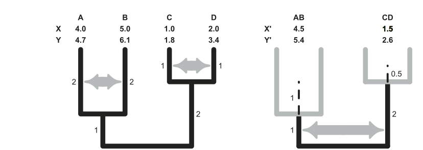
The algorithm runs iteratively from the tips to the root of the phylogeny, transforming n phenotypic measurements that are not independent in n–1 contrast that are statistically independent. Because phenotypic estimates at intermediate nodes (X’ and Y’) are not measured, but inferred from the tip data, divergence times employed to calculate these contrasts include an additional component of variance that reflects the uncertainty associated with these estimates. In practice, this involves lengthening the branches (dashed lines) by an amount that, assuming Brownian motion, can be calculated as:
(daughter branch length 1 × daughter branch length 2)
-----------------------------------------------------
(daughter branch length 1 + daughter branch length 2)

Contrasts results and statistical analysis
As a result, the association between the hypothetical phenotypic variables X and Y analyzed employing conventional statistics and independent contrasts may seem remarkably different. Because independent contrasts estimate phenotypic divergence after speciation and are expressed as deviations from zero (i.e., the daughter lineages were initially phenotypically identical), correlation and regression analyses employing contrasts do not include an intercept term and must be always calculated through the origin.

Note that the sign of each contrast is arbitrary; hence many studies have adopted the convention to give a positive sign to contrasts in the x-axis and invert the sign of the contrast in the y-axis accordingly (this procedure does not affect regression or correlation analyses through the origin). Even though the classic algorithm to calculate contrasts neglects important sources of uncertainty such as individual variation and measurement error, recent methods can account for these sources of error.
R/ape tutorial for independent contrasts
Independent contrasts drawbacks
- Tree needs to be fully bifurcating (otherwise, which against which for the contrast?)
- Data points (n-1) no longer represent species, but the differences between them (so, how to detect if any particular species or group is exceptional?)
- Also, how to do more complex modeling and hypothesis testing? Maybe there are better approaches?
An example case


Ordinary least squares
In an ordinary least squares (OLS) regression model, the relationship of a response variable Y to a predictor variable X1 can be given using the regression equation:

- b0 is the intercept value of the regression equation,
- b1 is the parameter estimate (the slope value) for the predictor
- ε is the residual error (i.e. for a given point, how far it falls off the regression line).
For a simple regression with one predictor (X), the slope of the regression line b1 is given by:

- n is the sample size
- Xi is the i th value of X (up to the last value Xn)
- X̄ represents the mean value of X (0.97)
- Likewise for Yi and Ȳ (1.30)
The intercept b0 then follows:

Generalizing the model: the variance-covariance matrix
In the case of OLS, the implicit assumption is that there is no covariance between residuals (i.e. all species are independent of each other, and residuals from closely related species are not more similar on average than residuals from distantly related species).
This (n x n) variance–covariance matrix is denoted as C, and for five species under the assumption of no phylogenetic effects on the residuals, it looks like:

- The first row and first column represent values from comparisons with the first species (in our case Uca chlorophthalmus), the second row and column with Uca crassipes, and so on.
- Hence, the diagonal elements (the line of values from top left to bottom right) represent the variance of the residuals, while the other off-diagonal elements equal zero, meaning there is no covariation among the residuals.
- When this variance–covariance structure is assumed, the results of GLS are the same as those of OLS (the contribution of C to the regression calculation essentially drops out).
Variance-covariance matrix from relatedness
- The key statistical issue with cross-species analyses is that species data points are non-independent because of their shared phylogenetic history.
- Consequently, the errors may also be non-independent or autocorrelated (residuals from closely related species may be similar).
- Hence, there will be covariation in residuals, which we must account for in our variance–covariance matrix, C.

- The expected covariance will be related to the amount of shared evolutionary history between the species. Hence, the diagonal elements (i.e. the variance elements) of the matrix are the total length of branches from the root of the tree to the tips. This will be the same for each cell if the phylogeny is ultrametric (i.e. all tips are the same distance from the root of the phylogeny), as it is in the case of our example
- The off-diagonal covariance elements represent the total shared branch length of the evolutionary history of the two species being compared. Hence, for U. chlorophthalmus and U. crassipes, we see that each species has independent (nonshared) branch lengths of 1. Conversely, the two species share 2 branch lengths in their evolutionary history back to the root of the tree. Consequently, the value entered into column 1–row 2 (and column 2–row 1) of the matrix is 2.
- We can repeat this for all the other species comparisons (e.g. U. sindensis and U. argillicola do not share any evolutionary history, so their expected covariance is 0) and produce the new expected variance–covariance matrix.
Phylogenetic Generalized Least Squares (PGLS) solution
When this new version of C is applied to the GLS calculation (e.g. with geiger), we eventually end with the PGLS solution:
log(propodus length) = - 0.276 + 1.616 x log(carapace breadth)

Categorical data and character analysis
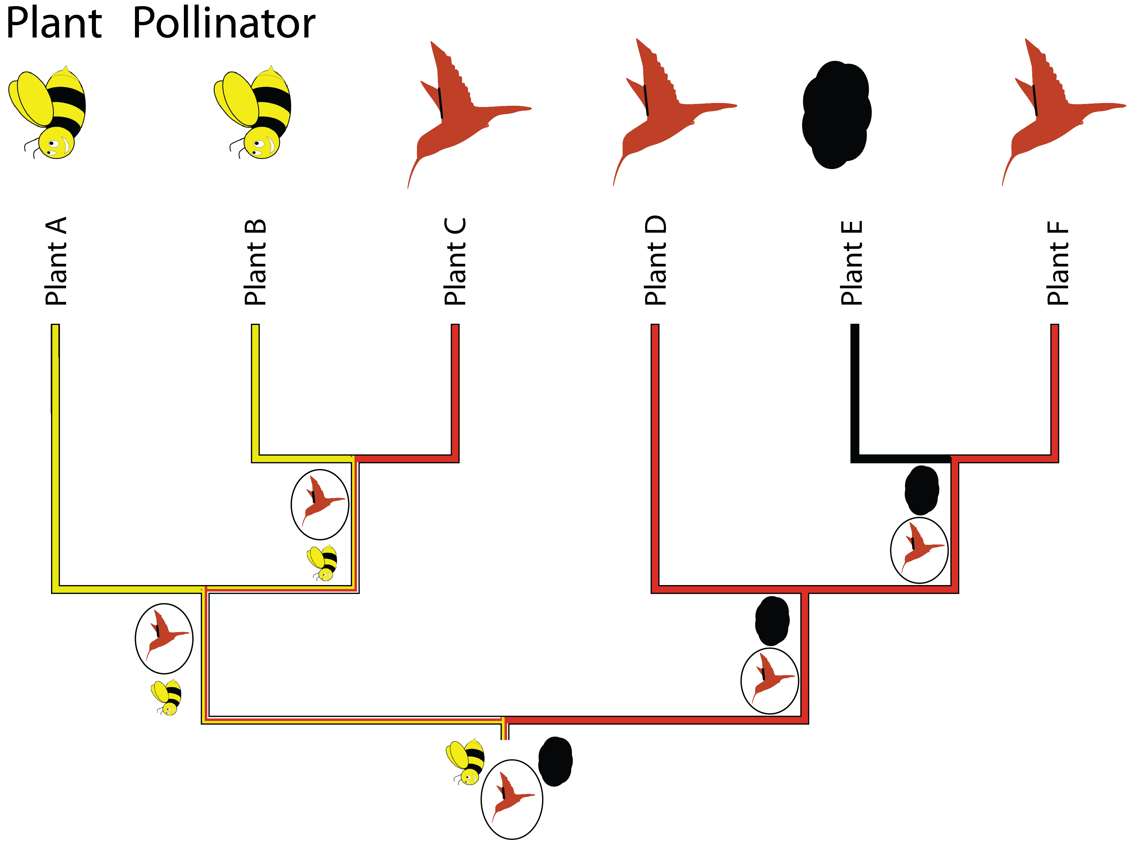
- Comparative analysis of discrete, categorical data (including biomolecular sequence data) requires other approaches to analyze, with implicit or explicit models for how discrete states change
- Under MP (as you might do in mesquite) the general assumption is that evolutionary change should be minimized (and then there can be constraints, e.g. about directionality)
- However, explicit models of state transitions allow for more kinds of hypothesis tests
Continuous-time Markov models
Transitions between states can be modeled as a rate matrix (Q). For example, for a character with two states (i and j), matrix looks like this:
| i | j | |
|---|---|---|
| i | 1-qij | qij |
| j | qji | 1-qji |
- The transition rate for i→j is qij
- A state either changes or it doesn’t: the rows must sum, hence the rate for i→i (i.e. no change) is 1-qij
- P(j,i,t) is the probability that a branch beginning in state i ends in state j, after time period t.
- For a given variable, P(j,i,t) will take only two forms for branches leading to the tips of the tree because j will be constant (it’s what we observe at the tips).
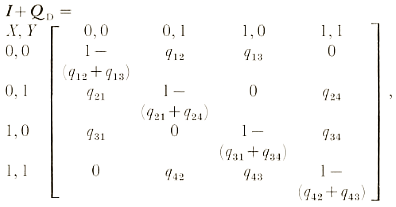
- For all other branches both j and i can vary from 0 to 1 so four possibilities arise in each variable (0→0, 0→1, 1→0, 1→1).
- Assume that we have two characters (X and Y), then the likelihood (L(I)) for this tree will be given by:


Likelihood
Quick recap
- Probability is used before data are available to describe plausibility of a future outcome, given a value for the parameter.
- Likelihood is used after data are available to describe plausibility of a parameter value.
The likelihood framework
- Likelihood values for different combinations of parameters (e.g. constraints on the Q matrix, alternative tree topologies) can be compared in hypothesis testing
- Maximum likelihood estimates obtain point estimates of the parameter values (e.g. tree shape) that maximize the likelihood
- Correlated traits can be tested by expanding the Q matrix:
Here is a tutorial that applies these concepts using the R package geiger.