mebioda
Querying the EoL trait bank

The Encyclopedia of Life is a web project that aims to provide
global access to knowledge about life on earth. It does this by constructing a web
page for each species and aggregating information from a variety of sources on that
page. As such, the way species are uniquely identified is by their
page_id. For example, the page_id of the Sea Otter
is 46559130, as you can see in the URL of the page.
Exercise 1: find the
page_idof your model organism on the EoL website
Triples and subjects
You will notice that for many species (probably your model organism as well) there is a tab called data on the species page. This leads to all the trait data that are available on the EoL website. Each individual trait value has a number of different bits of information associated with it:
- Where the information originally came from
- What the name of the trait is
- What the trait value is
- More detailed information when you expand the record by clicking the triangle
For example, a value for the trait geographic distribution includes might be Japan,
on the basis of a number of observations recorded in the Japan Species List. The
basic fact that the geographic distribution of this species includes Japan can be
represented as a ‘triple’:
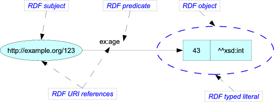
A triple is like a machine-readable sentence, and it is called that way because it
consists of three parts: the subject, the predicate, and the object. For the sentence
‘the sky is blue’, the subject is ‘the sky’, the predicate is ‘is’, and the object
is ‘blue’. Likewise, the picture shows a subject (http://example.org/123), a predicate
(ex:age), and an object (43). The triple thus means to say that whatever is identified
by the URL has an age of 43.
Exercise 2: for any EoL trait record, what is the subject?
Predicates
On several occasions during the course we’ve discussed the importance of making it unambiguously clear what we mean when we use a certain term in our data. For example, when you combine different data tables, do columns with the same name automatically mean they hold the same data? Are columns with different names necessarily different? It is impossible to say unless the terms that we use are anchored on a globally unique definition. We may have used the word ‘ontology’ or ‘controlled vocabulary’ for this.
The EoL trait bank uses this in a big way. Every predicate (so, every term about a
species, such as geographic distribution includes) is anchored on an ontology. Many
predicates are basically invented and defined by EoL itself, but others are borrowed from
external ontologies. This is a good idea, because we are only going to be able to
link up on the web of data if there is a shared agreement across different data sources
on what our predicates mean. And to make sure that we uniquely identify the predicate,
it is given a URI (a special type of URL that is used for identifying things. It doesn’t
necessarily lead to a web page when you try to load it, though it might. The main
purpose is just to create an identifier.)
Exercise 3: in the trait data for a model plant, look for the predicate ‘Leaf Complexity’. What is its URI? What ontology does it come from?
Objects
The third part of a triple is the object. In the picture of the triple, the object is
the literal value 43. It is possible that this is ambiguous, because we don’t know
right away what the unit is here. Perhaps it is the case that the definition of the
predicate ex:age specifies this, for example by stating that this is age in years
(as opposed to days, millions of years, milliseconds). On other occasions we have
already seen how this is commonly specified, for example when we collected occurrence
data: the terms dwc:decimalLatitude
and dwc:decimalLongitude are clear
enough. (So, yes, GBIF uses ontologies as well, and so do BoLD, GenBank, and many other
databases with biodiversity data.)
In many cases it becomes unwieldy, or really impossible, to cram information about the object into the predicate such that the object can remain a literal value. Instead, the object also becomes a term from an ontology. For example, the territorial extent of Japan has varied over the years, so whether a species includes Japan in its geographical distribution depends on what is meant by that, which EoL clarifies by using this globally unique anchor.
Exercise 4: for the trait value ‘green’ (for example as the object of the triple where the predicate is ‘leaf color’), what is the definition? What ontology does that come from?
So, there are literal objects, which are usually numbers (counts, measurements), and there are objects that themselves are ontology terms. You can imagine that those objects can, in turn, become subjects of other statements: there are many things that can be said about Japan, or about the color green, so they can naturally become subjects of other triples. And the objects of those triples can in turn become the subjects of others, and so on. Within and across data resources, this creates a very large network (or ‘graph’) of data:
Data services
In the following exercises, we are going to try out some queries on the web service interface of EoL. This is similar to the requests we placed on the web server for DNA barcodes (BoLD), where we downloaded JSON and FASTA data. In this case, more flexible and powerful queries can be run, but they require you to log in. If you don’t have one yet, make an account on the EoL.org website and make sure you are logged in. Then continue with the following sections.
Graph databases
As we saw in the first week, networks (or “graphs”) can be stored in relational databases: a phylogenetic tree is a graph - a DAG - that can be traversed using recursive queries. These queries are basically of the form Q1: “get me the children of this node”, Q2: “now get me the children of the children”, and so on. This quickly becomes tedious, and it doesn’t work in the same way when there are cycles in the tree, for example when a node has multiple ancestors.
A sensible solution is to not use a relational database, but a graph database. For the network of linked data on the web, graph databases offer several advantages over traditional, relational databases. In a graph database you search for patterns without having to specify how these come about (a relational SQL database requires you to be more explicit about what joins with what).
The most commonly used graph database right now is probably Neo4J, and it is the one that EoL uses. Neo4J has its own query language, cypher.
It looks a bit like the standard language SQL that we saw in weeks 1 and 2, but it’s a language specific to Neo4J and it uses ASCII art to represent relations:
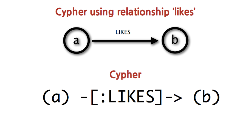
The above picture shows that “a likes b” (what’s the subject here? The predicate? The object?),
where (a) and (b) are now nodes (vertices) in the graph, and -[:LIKES]-> is the
relationship between them (an edge connecting the nodes in the graph). So how does this
work with the Linnean taxonomy? Assume the following:
- Taxon nodes (really, pages) in the EoL graph have a
page_id - They also have a
canonicalname (i.e. the accepted taxonomic name) and aparent - The
parentattribute creates a pattern just like the-[:LIKES]->thing
With this information we can run a query where we can get all the ancestors of the Sea Otter in one go (and without clever, pre-computed index columns). The following allows you to run that query. It is going to return JSON data, so it’s a good idea to have a browser extension that allows you to view JSON (chrome plugin, firefox plugin) before you run the query:
To unpack the query above, line by line:
- Give me all the
ancestorpages with which theorigin(identified bypage_id46559130) has a-[:parent*]->relation. The clever thing here is that theparentrelation is transitive because of the extra asterisk *, i.e. parent-of-parent also matches (and parent-of-parent-of-parent, etc.) - For any of these ancestors, give me their parent. This clause is optional, because not all ancestors have a parent. Which one doesn’t?
- For the matching ancestors, give me the
page_idand thecanonical, and theparent_idof its parent (this is allowed to be ‘null’) - Limit the results to 100 ancestors.
Exercise 5: Now try the same thing with your model organism’s page_id
Querying for literal trait data
From the EoL documentation
it looks like a (Page), i.e. a taxon, can have zero or more -[trait]-> patterns, which
point to a (Trait) node. The trait node in turn points to a (Term) node with which it has a
-[:predicate]-> relation (i.e. what is the specific predicate term that we use for this trait),
and optionally another (Term) node that gives the measurement units of the literal trait value.
Here is an example to fetch a single trait triple for the Sea Otter:
Line by line, the query roughly goes like this:
- Give me the traits
tfor a pagep - For those traits
t, go on and give me the predicate termpred - Do this given that
page_idof pagepis 46559130 and the predicate has this URI - If the trait also has a units term, give me that as well
- Return the triple, i.e. subject
p.canonical, predicatepred.name, objectt.measurementand add theunits.name - I only want the first result
Exercise 6: Run the query with your model organism’s page_id. Do you get any results? If not, why not?
Exercise 7: Run the query with your model organism’s page_id, but increase the
LIMIT(like, set it to 100, for example), and remove the second part of theWHEREclose, so without the part from theANDstatement onwards on line 3.
Because we’ve removed the restriction to a specific predicate in Exercise 7, we get whatever predicates
are available. However, many of them have no literal object value. Why? Because the object is not a
literal measurement (such as the body mass) but something else, such as an ontology term for a habitat type.
Querying object trait data
In the case of the literal values it made sense to have the trait specify a relation to a
(units:Term) that contained the name of the measurement unit (g, mm, ångström, whatever).
For trait values that are objects themselves, it works a bit differently. Here, the relevant
information about the trait value is contained within the object, by way of a term definition
(what is Japan? What is green?). The trait therefore has a relation that is defined
as -[:obj_term]-> instead of -[:units_term]->. The example below produces the first
object term for the Sea Otter:
Exercise 8: Run the query for your model organism and increase the limit (100?)
Exercise 9: Refine the query by adding a
AND pred.uri = "<uri>"to theWHEREline, and put in place ofthe URI for [geographic distribution includes]
Notice how there are “duplicate” results? They are trait values from different sources, or
otherwise different in some way when you inspect the full record on the website. If all we want
is the full set of distinct geographic areas that the species includes in its range we
can modify the query to make it RETURN DISTINCT ... (on the fifth line).
Exercise 9: Refine the query to make it return distinct records for the geographic localities.
Exporting data
If that worked so far, you would have got all the distinct areas, but perhaps also a null
value, because the presence of the -[:object_term]-> pattern was optional. We can make
that a required part of the query. Notice how the clause that was on the fourth line
(OPTIONAL MATCH <clause>) has now moved to the third line as part of the MATCH
statement:
Notice how there is now a button where you can switch between output formats? If you click CSV the data will be produced as a table, such as the one here. A logical next step for some of you in relation to the MAXENT analyses would have been to associate the different localities with shape files. You would then have a filter to keep only those occurrences that fall within the shapes for cleaning your data. With a spatial join, for example. But not today. Done.
Read more about EoL queries on their repository here.