mebioda

Species delimitation with DNA barcodes

Species concepts and delimitation intro

The following slide show provides an overview of species concepts and the application of species delimitation techniques to natural history collection specimens:

Species delimitation - species limits and character evolution

Barcode Index Number (BIN)

Ratnasingham, S & Hebert, PDN 2013. A DNA-Based Registry for All Animal Species: The Barcode Index Number (BIN) System. PLoS ONE 8(7): e66213 doi:10.1371/journal.pone.0066213 (pdf)

BIN divergence thresholds

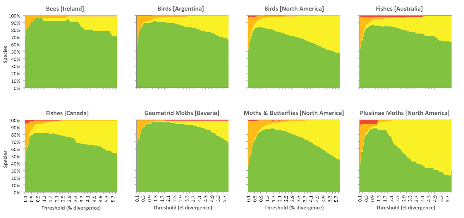
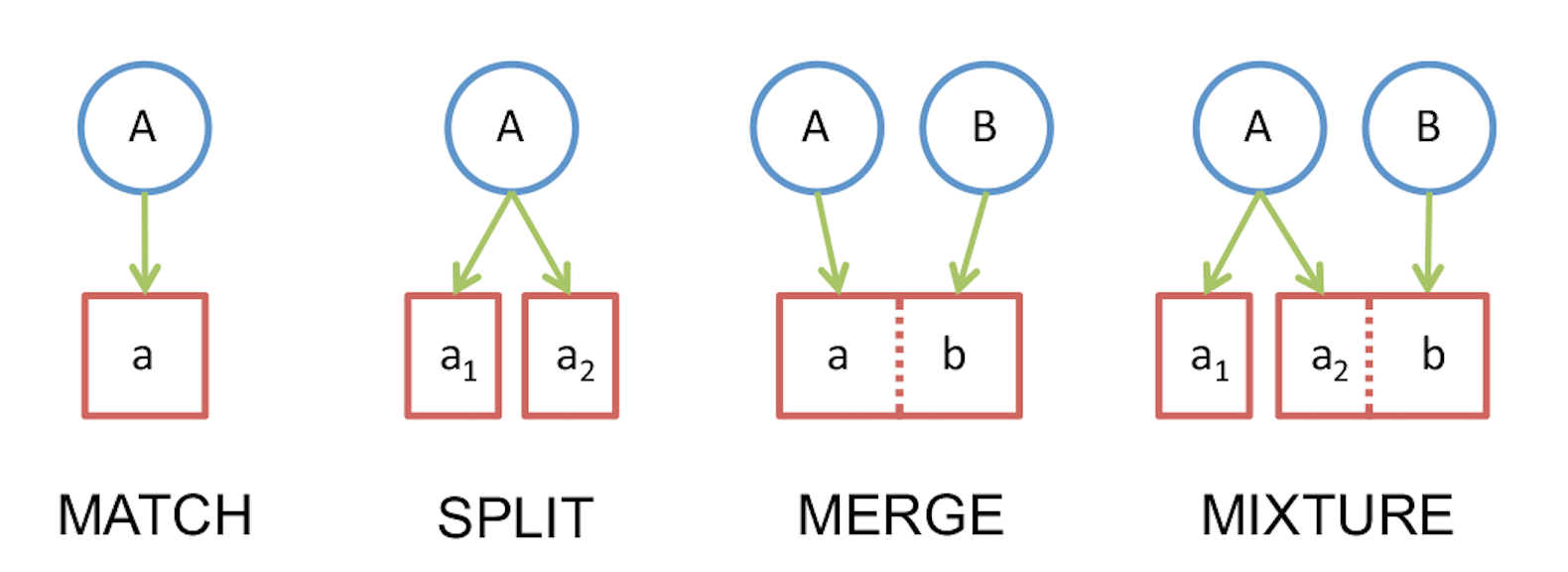
Correspondence between species present in eight datasets and OTUs recognized through single linkage clustering with sequence divergence thresholds ranging from 0.1–6.0%.

Green indicates the number of OTUs whose members perfectly match species
Yellow shows those that merge members of two or more species
Orange indicates cases where a species was split into two or more OTUs
Red represents a mixture of splits and merges

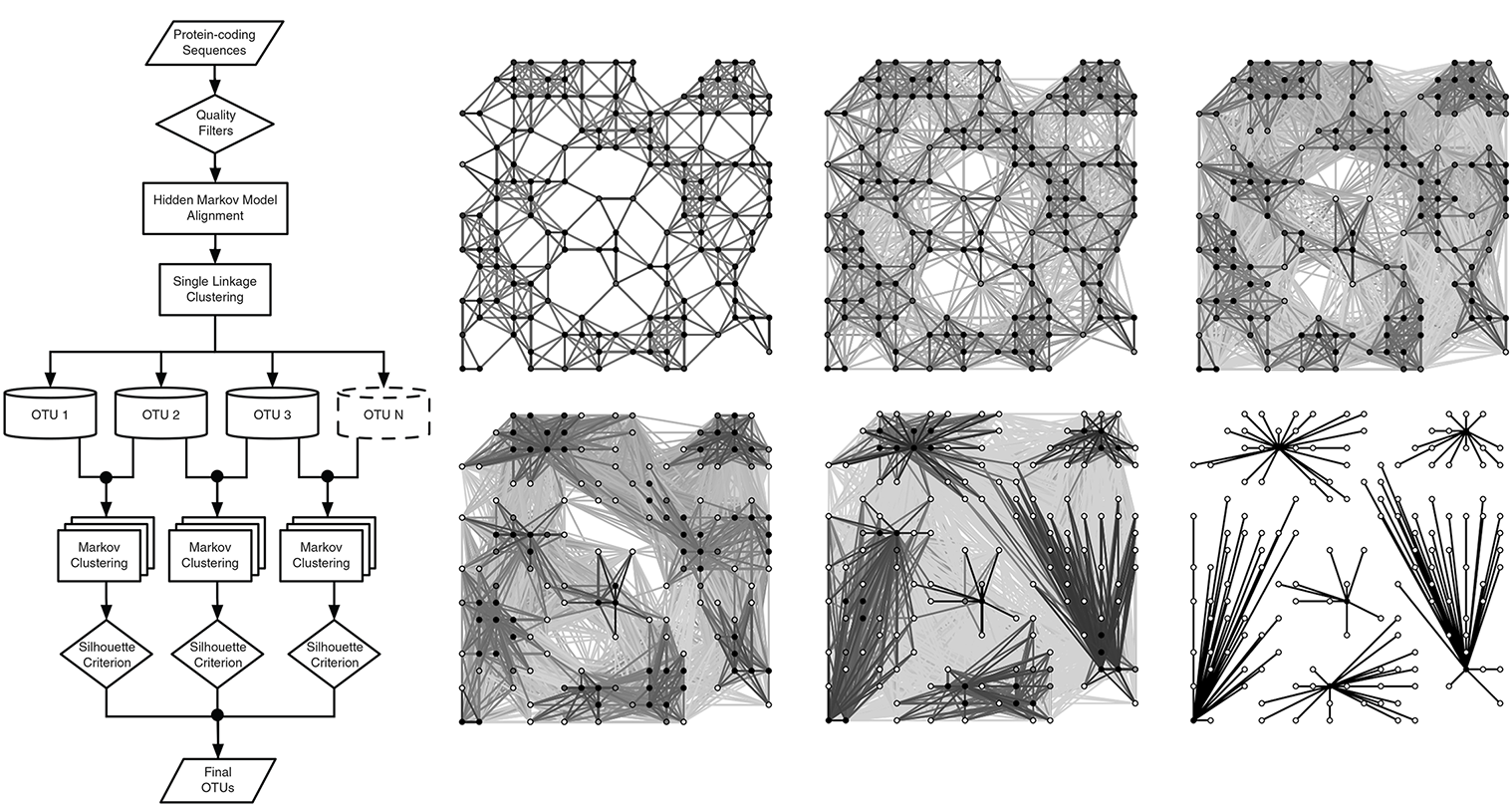
BIN pipeline

HMM alignment uses a profile of the COI marker protein
SLC connects sequences by distance, but creates ‘long’ graphs
MCL iteratively looks for ‘attractors’ within the graphs and re-clusters around them

Automatic Barcode Gap Discovery (ABGD)

Puillandre N, Lambert A, Brouillet S & Achaz G 2012. ABGD, Automatic Barcode Gap Discovery for primary species delimitation. Mol Ecol. 21(8): 1864-77 doi:10.1111/j.1365-294X.2011.05239.x (pdf)

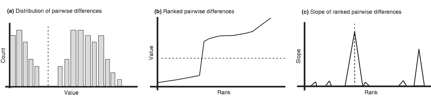
(a) A hypothetical distribution of pairwise differences. This distribution exhibits two modes. Low divergence being presumable intraspecific divergence, whereas higher divergence represents interspecific divergence.
(b) The same data can be represented as ranked ordered values.
(c) Slope of the ranked ordered values. There is a sudden increase in slopes in the vicinity of the barcode gap. The ABGD method automatically finds the first statistically significant peak in the slopes.

The ABGD command line tool

$ curl -L -O http://wwwabi.snv.jussieu.fr/public/abgd/last.tgz
$ tar xzvf last.tgz
$ cd Abgd
$ make
$ export PATH="${PATH}":`pwd`

We should now have an executable called abgd on the $PATH. This accepts aligned FASTA as input, so let’s analyze one of the files we have:

# inside w1d3 folder
$ mkdir Danaus_ABGD
$ abgd -o Danaus_ABGD -a Danaus.mafft.fas

Resulting files, showing the barcode gap inflection point:

Generalized Mixed Yule Coalescent (GMYC)

Fujisawa T & Barraclough TG. 2013. Delimiting Species Using Single-Locus Data and the Generalized Mixed Yule Coalescent Approach: A Revised Method and Evaluation on Simulated Data Sets Systematic Biology 62(5): 707–724 doi:10.1093/sysbio/syt033 (pdf)

Separate evolutionary lineages diversify according to processes such as the Yule (pure birth) model, the simplest one.
Gene copies coalesce according to population genetic processes (e.g. the rate is proportional to the effective population size).
The GMYC method looks for the MLE of where the coalescent process took over from the lineage diversification process.

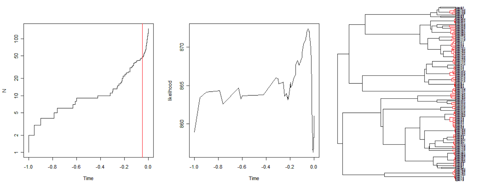
The GMYC web service

The analysis can be performed through a web service, and results for the Danaus consensus tree in the following clusters:

number of ML clusters: 13 (CI: 11-14)
number of ML entities: 15 (CI: 13-16)

Which are distributed across the clades near the tips:

How many (using line count, wc -l) distinct taxonomic names do we have in the alignment:

$ grep '>' Danaus.mafft.fas | cut -f 1 -d '-' | sort | uniq | wc -l
      15

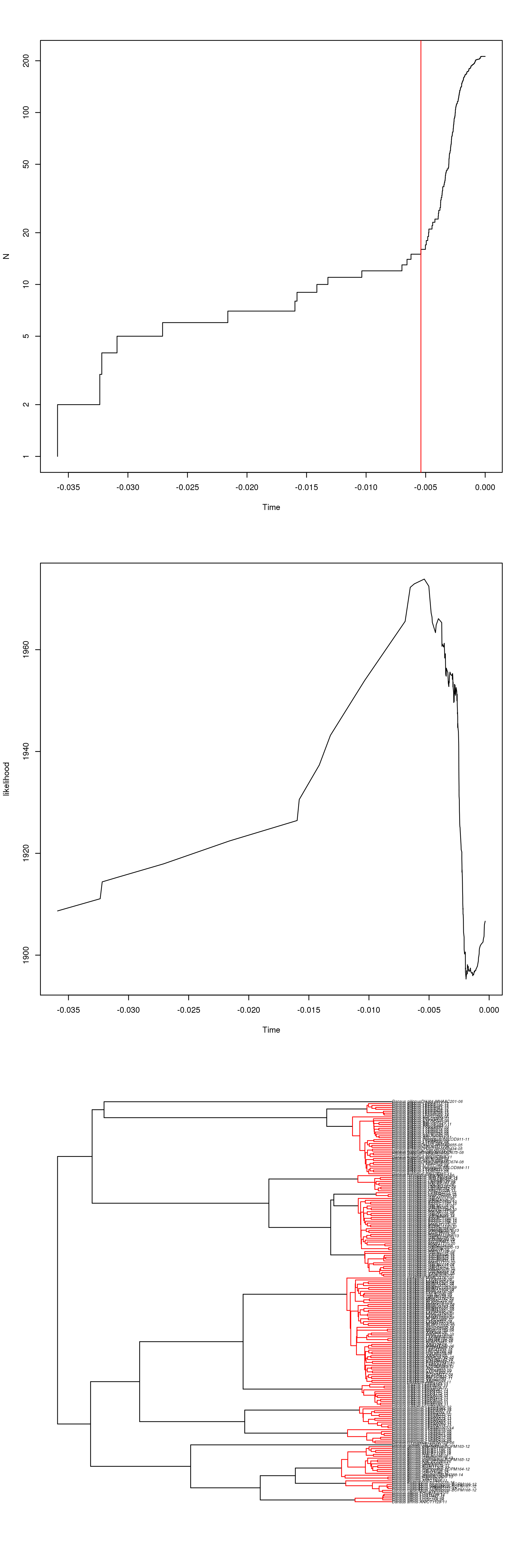
Poisson Tree Process (PTP)

J Zhang, P Kapli, P Pavlidis, A Stamatakis 2013. A general species delimitation method with applications to phylogenetic placements. Bioinformatics 29(22): 2869–2876 doi:10.1093/bioinformatics/btt499

Is tree-based, but doesn’t require ultrametric (clock-like) trees
Uses phylogenetic distance as a proxy for substitutional difference, expecting to see different classes of distances produced by different Poisson processes
Has a Bayesian implementation that produces support values for clusterings

Using the same tree as for GMYC on the bPTP web server obtains an MLE of 16 species with potential for (far) greater splitting:

Accptance rate: 0.69020000000000004 
Merge: 49798 
Split: 50202 
Estimated number of species is between 14 and 135 
Mean: 78.03

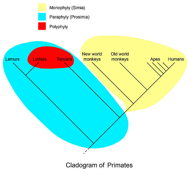
Monophyly, polyphyly, paraphyly

Mutanen, M et al. 2016. Species-Level Para- and Polyphyly in DNA Barcode Gene Trees: Strong Operational Bias in European Lepidoptera, Systematic Biology 65(6): 1024–1040 doi:10.1093/sysbio/syw044

So how are the putative species from BoLD actually entangled?

For each taxon:

Collect all tips that belong to it
Find the MRCA for the collected tips
Collect all descendants of the MRCA. If this set is identical to the set of step 1. then the taxon is monophyletic and the analysis moves on to the next taxon.
Collect all nodes that subtend tips from the focal taxon as well as at least one other taxon and sort these by their post-order index.
Group the collected, sorted nodes into distinct root-to-tip paths. Internal nodes that are nested in each other are identified (and collected in the same group) by checking that the pre-order index of the focal node is larger, and the post-order index of the focal node is smaller than that of the next node in the sorted list. If there is more than one distinct root-to-tip path (i.e., group), the taxon is considered polyphyletic, otherwise paraphyletic.
For each first (i.e. most recent) node in each group, collect all subtended species. The union of these sets across groups forms the set of entangled species.

$ curl \
  -F "infile=@BEAST/Danaus.consensus.trees.nwk" \
  -F "format=newick" \
  -F "separator=-" \
  -F "astsv=true" \
  -F "cgi=true" \
  http://monophylizer.naturalis.nl/cgi-bin/monophylizer.pl > Danaus.monophyly.tsv

Which produces a spreadsheet that identifies the exact matches (i.e. monophyletic) and where there is entanglement among species (i.e. paraphyletic or polyphyletic).

This site is open source. Improve this page.